Using plotmath in ggplot objects • Adventures in data

This one will be quick.

I always struggled to use R math expressions in ggplot objects.
The API looks quite inconsistent, as the specification to activate plotmath parsing changes depending on which object is to be plotted.

So here’s a short post to resume a few techniques and a few tips!

More information can be found in the ggplot2 wiki.

Data

Let’s generate some data: this is a standard data frame, which contains expressions that can be interpreted as plotmath.


library(dplyr)
library(ggplot2)

df <- data.frame(
   var = c('alpha', 'beta', 'X[1]', 'X[2]', 'X[3]'), 
   power = paste0('y^', 1:5),
   value = 1:5, 
   letter = c(rep('alpha', 3), rep('omega', 2))
)
df
##     var power value letter
## 1 alpha   y^1     1  alpha
## 2  beta   y^2     2  alpha
## 3  X[1]   y^3     3  alpha
## 4  X[2]   y^4     4  omega
## 5  X[3]   y^5     5  omega

For example, for a given statistical unit one might have observed the values in df$value corresponding to the variables in df$var. (disregard the other columns, for now).
To put that in tidy form, one would have had the following data frame:

df_simple <- df$value %>% as.matrix() %>% t() %>% as.data.frame()
colnames(df_simple) <- df$var
df_simple
##   alpha beta X[1] X[2] X[3]
## 1     1    2    3    4    5

Notice that the columns are not easily accessible, one has to use the backticks to escape the [ operator:

df_simple$alpha
## [1] 1
df_simple$`X[1]`
## [1] 3

Plotting the problem

The previous data frame could be plotted using standard ggplot tools (notice again the backticks):

ggplot(df_simple) + geom_point(aes(x = `X[1]`, y = `X[2]`))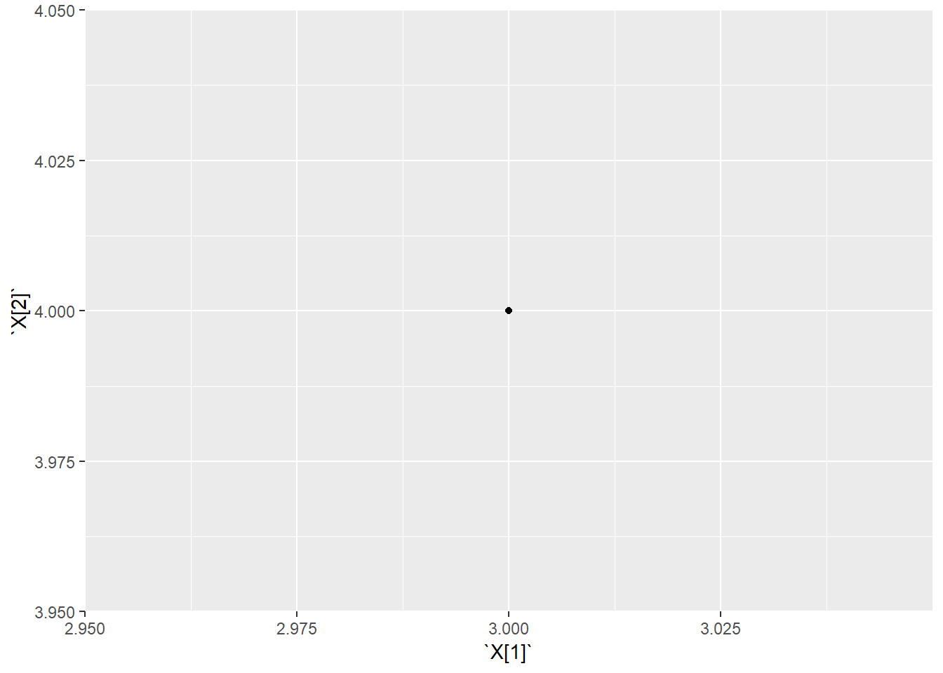

Looks good (ok, it is only one point, but the example holds for any data frame with more rows).
However, the axes are poorly named.

The same happens if we use the first data frame to produce a more complex plot, using more ggplot functions.
An example with facets, labels and discrete scales:


ggplot(df) +
   facet_wrap(~ letter) +
   geom_point(aes(x = var, y = value, col = power)) +
   geom_label(aes(x = var, y = value, col = power, label = power), show.legend = FALSE)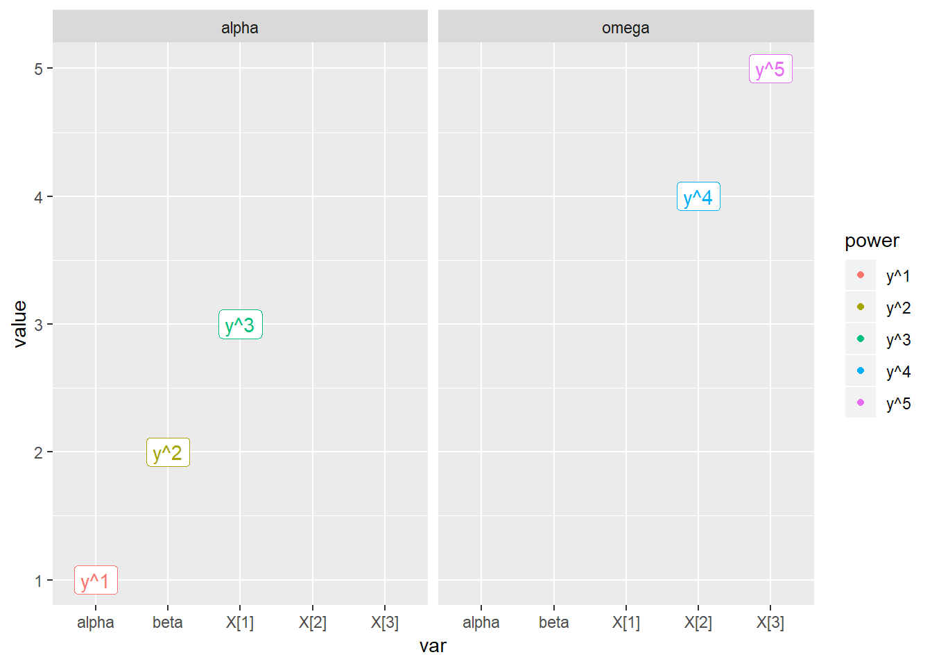

Again, all labels could be interpreted as plotmath expressions.

The solution

Facet labels

To interpret facet labels as plotmath expressions, ggplot2 provides the function label_parsed:


ggplot(df) +
   facet_wrap(~ letter, labeller = label_parsed) +
   geom_point(aes(x = var, y = value, col = power)) +
   geom_label(aes(x = var, y = value, col = power, label = power), show.legend = FALSE)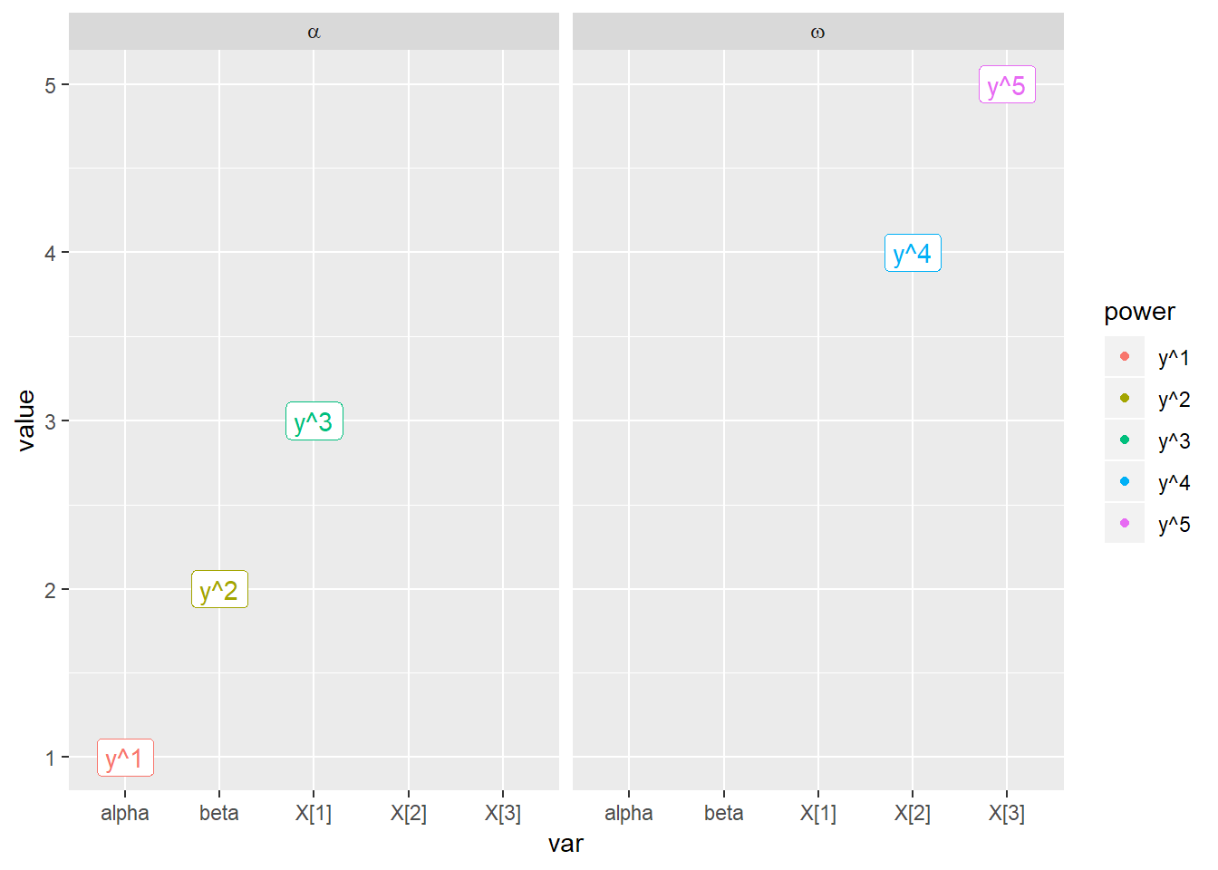

Text and label geoms

This is easy: geom_label and geom_text support the argument parse = TRUE:

ggplot(df) +
   facet_wrap(~ letter, labeller = label_parsed) +
   geom_point(aes(x = var, y = value, col = power)) +
   geom_label(aes(x = var, y = value, col = power, label = power), show.legend = FALSE, parse = TRUE)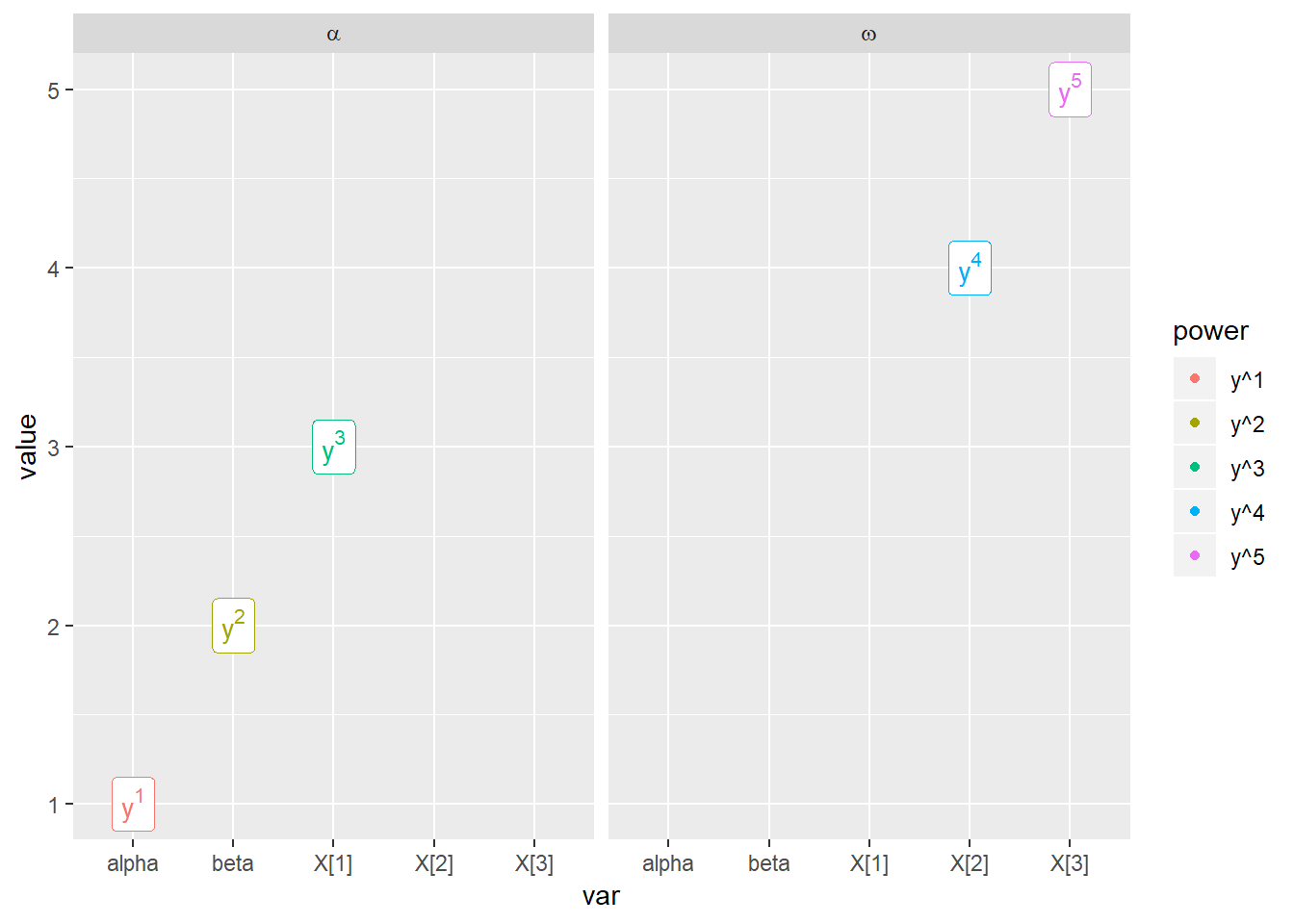

Discrete scales: axis ticks, color values

Discrete scales are more complicated: one can supply a vector of breaks (i.e. numeric values specifying where the scale is broken, in data units), and a vector of labels (a character vector which is used to label each break).


x_breaks <- levels(df$var)
x_labels <- parse(text = x_breaks)

ggplot(df) +
   facet_wrap(~ letter, labeller = label_parsed) +
   geom_point(aes(x = var, y = value, col = power)) +
   geom_label(aes(x = var, y = value, col = power, label = power), show.legend = FALSE, parse = TRUE) +
   scale_x_discrete(breaks = x_breaks, label = x_labels)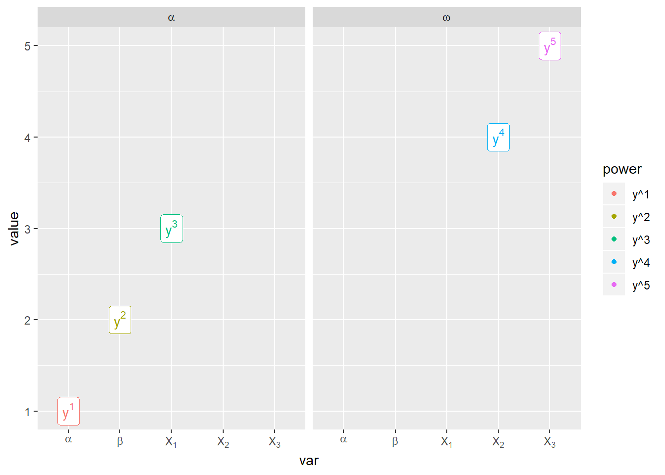

A much faster alternative is to use the fact that a function can be passed as the argument label for discrete scales. This function “takes the breaks as input and returns labels as output”.
So let’s define the function label_parse:

label_parse <- function(breaks) {
   parse(text = breaks)
}

The previous example can be highly semplified:

ggplot(df) +
   facet_wrap(~ letter, labeller = label_parsed) +
   geom_point(aes(x = var, y = value, col = power)) +
   geom_label(aes(x = var, y = value, col = power, label = power), show.legend = FALSE, parse = TRUE) +
   scale_x_discrete(label = label_parse)

It’s the same also for discrete color scales:

ggplot(df) +
   facet_wrap(~ letter, labeller = label_parsed) +
   geom_point(aes(x = var, y = value, col = power)) +
   geom_label(aes(x = var, y = value, col = power, label = power), show.legend = FALSE, parse = TRUE) +
   scale_x_discrete(label = label_parse) +
   scale_color_discrete(label = label_parse)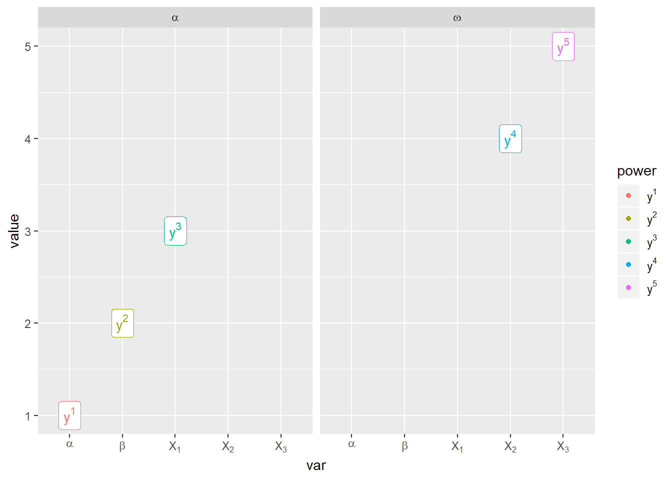

More complicated expressions

For expressions which merge plotmath and plain text, a shortcut is not simple, one has to use some more plotmath operators like paste.
See this (or many others!) blog post for examples.

Here, in df$exp and df$var I use the ~ operator to insert a space between a text string (in double quotes) and math symbols (this is equivalent to the paste operator):

df_2 <- data.frame(
   var = c('"Variable" ~ X[1]', '"Variable" ~ X[2]', '"Variable" ~ X[3]', '"Variable" ~ X[4]'),
   exp = c('"Linear:" ~ a*X + b', 
           '"Quadratic:" ~ a*X^2 + b*X + c', 
           '"Mean:" ~ mu', 
           '"Bilinear:" ~ a[1]*X + a[2]*Y'),
   val = 1:4
)

ggplot(df_2) +
   geom_point(aes(x = var, y = val)) +
   geom_label(aes(x = var, y = val, label = exp), show.legend = FALSE, parse = TRUE) +
   scale_x_discrete(label = label_parse)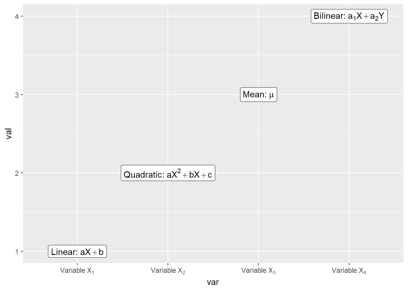

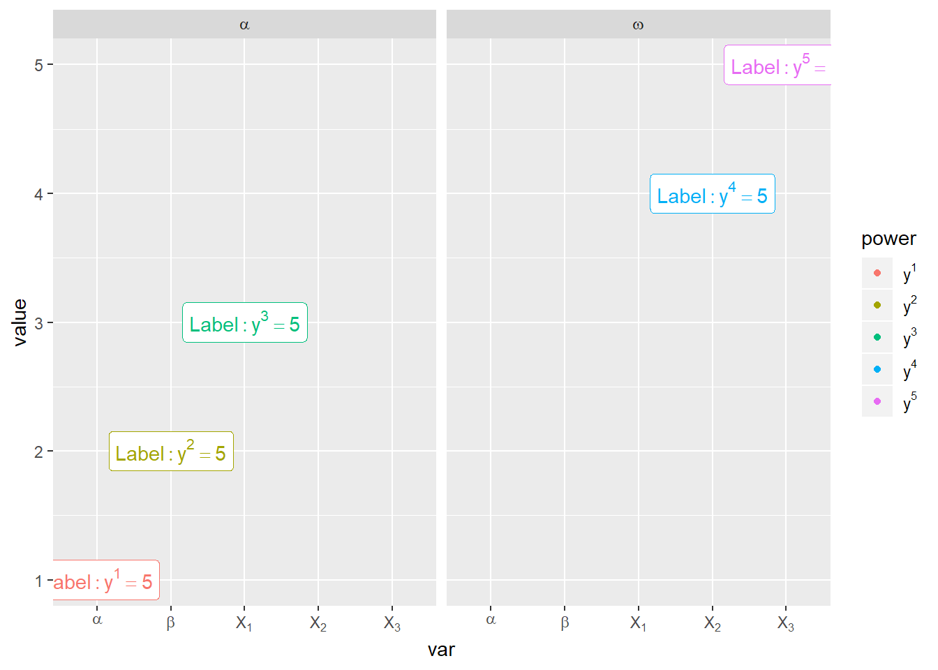
If one wants to insert actual values for parameters, then I think one is forced to build the expression manually, or to use bquote:

ext_val <- 5

ggplot(df) +
   facet_wrap(~ letter, labeller = label_parsed) +
   geom_point(aes(x = var, y = value, col = power)) +
   geom_label(aes(x = var, y = value, col = power, label = paste("Label:", power, "==", ext_val)), show.legend = FALSE, parse = TRUE) +
   scale_x_discrete(label = label_parse) +
   scale_color_discrete(label = label_parse)